An introduction to self-adaptive cooperative enhanced scatter search (saCeSS) in PyScat
Goals:
Introduce the concepts of self-adaptive cooperative enhanced scatter search (saCeSS)
Show how to use the
pyscat.SacessOptimizerand introduce its hyperparameters
It is recommended to read the eSS introduction first.
The PyScat scatter search implementations are based on the following publications:
Jose A. Egea, Eva Balsa-Canto, María-Sonia G. García, and Julio R. Banga. Dynamic optimization of nonlinear processes with an enhanced scatter search method. Industrial & Engineering Chemistry Research, 48(9):4388–4401, April 2009. doi:10.1021/ie801717t.
David R. Penas, Patricia González, Jose A. Egea, Ramón Doallo, and Julio R. Banga. Parameter estimation in large-scale systems biology models: a parallel and self-adaptive cooperative strategy. BMC Bioinformatics, January 2017. doi:10.1186/s12859-016-1452-4.
[1]:
import logging
from pprint import pprint

import matplotlib.pyplot as plt
import numpy as np

from pyscat import SacessOptimizer, get_default_ess_options
from pyscat.plot import plot_sacess_history

np.random.seed(1337)
Set up problem
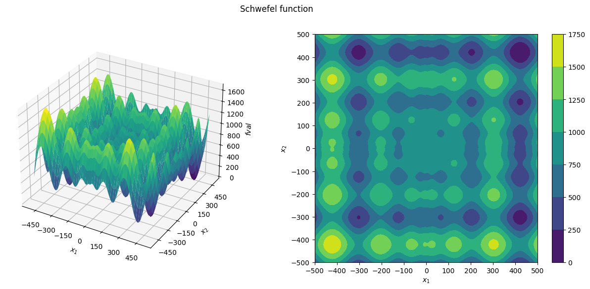
To run any optimization, we first need to specify the optimization problem. PyScat currently heavily relies on the pyPESTO framework and requires a pypesto.Problem. For this demo, we use the Schwefel function which is one of the examples included in PyScat:
[2]:
from pyscat.examples import plot_problem, problem_info, xyz

cur_problem_info = problem_info["Schwefel"]

problem = cur_problem_info["problem"]

plot_problem(problem, title="Schwefel function")
[3]:
# generate data for plotting
X, Y, Z = xyz(problem)


# plotting function for our objective landscape
def plot_f(ax=None):
    """contour plot"""
    if ax is None:
        ax = plt.gca()

    c = ax.contourf(X, Y, Z, cmap="viridis")
    plt.colorbar(c, ax=ax, label="fval")
    ax.set_xlabel("$x_1$")
    ax.set_ylabel("$x_2$")
Self-Adaptive Cooperative Enhanced Scatter Search (saCeSS)—SacessOptimizer
Motivation
eSS makes it difficult to balance exploration and intensification
eSS hyperparameters are difficult to tune
eSS itself offers limited room for parallelization to reduce walltime
Approach
cooperative: eSS (
ESSOptimizer) instances with different degrees of exploration versus intensification are running concurrently and exchange promising solutionsasynchronous communication: non-blocking exchange of solutions
self-adaptive: concurrent eSS instances exchange hyperparameters
Implementation
Several SacessWorker are running in parallel, controlled by a SacessManager that handles global state, each running an instance of ESSOptimizer.
Optimization with default options
For SacessOptimizer there are plenty of hyperparameters that can be tuned, but for a start we just use the default settings. The only options that have to be specified are:
the number of workers
num_workers(i.e., the numberESSOptimizerinstances that will run in parallel)the walltime limit
max_walltime_s
[4]:
optimizer = SacessOptimizer(
    problem=problem,
    num_workers=6,
    max_walltime_s=2,
    sacess_loglevel=logging.WARNING,
)
result = optimizer.minimize()
[5]:
# Generate default options for the individual eSS instances
ess_options = get_default_ess_options(
    num_workers=6, dim=problem.dim, local_optimizer=False
)
print("Options for the individual eSS instances:")
pprint(ess_options)

# Initialize and run the optimizer
sacess = SacessOptimizer(
    problem=problem,
    ess_init_args=ess_options,
    max_walltime_s=2,
    mp_start_method="fork",
    sacess_loglevel=logging.WARNING,
)
result = sacess.minimize()
result
Options for the individual eSS instances:
[{'balance': 0.0, 'dim_refset': 5, 'local_n1': 1, 'local_n2': 1},
 {'balance': 0.0, 'dim_refset': 5, 'local_n1': 1000, 'local_n2': 1000},
 {'balance': 0.25, 'dim_refset': 5, 'local_n1': 10, 'local_n2': 10},
 {'balance': 0.5, 'dim_refset': 5, 'local_n1': 20, 'local_n2': 20},
 {'balance': 0.25, 'dim_refset': 6, 'local_n1': 100, 'local_n2': 100},
 {'balance': 0.25, 'dim_refset': 6, 'local_n1': 1000, 'local_n2': 1000}]
[5]:
<pypesto.result.result.Result at 0x701df1d20550>
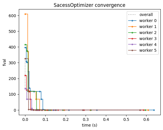
Visualize the optimization trajectory across iterations:
[6]:
plot_sacess_history(sacess.histories)
plt.show()
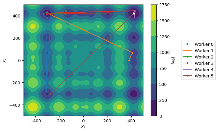
plot_f()
for i, history in enumerate(sacess.histories):
h = np.vstack(history.get_x_trace())
plt.plot(h[:, 0], h[:, 1], marker=".", label=f"Worker {i}")
plt.legend(loc="center left", bbox_to_anchor=(1.3, 0.5))
r = np.vstack(result.optimize_result.x)
plt.scatter(
r[:, 0], r[:, 1], c="white", marker="*", label="Reported optimum", zorder=5
)
plt.show()
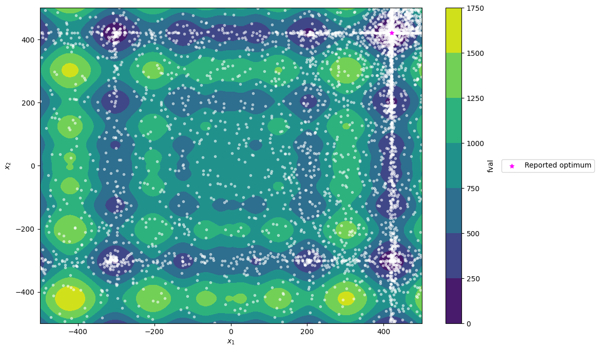
Visualize exploration of the parameter space (the API is experimental, and recording all visited points is usually quite memory intensive):
[7]:
from pyscat.eval_logger import EvalLogger

el = EvalLogger()
with el.attach(problem):
    sacess = SacessOptimizer(
        problem=problem,
        ess_init_args=ess_options,
        max_walltime_s=1,
        mp_start_method="fork",
        sacess_loglevel=logging.WARNING,
    )
    result = sacess.minimize()
[8]:
# extract traces
x_trace = np.array([x for x, _ in el.evals])
fx_trace = np.array([fx for _, fx in el.evals])

plot_f()
# plot all visited points
plt.scatter(x_trace[:, 0], x_trace[:, 1], marker=".", alpha=0.5, c="w")
# plot optimum
plt.scatter(
    result.optimize_result.x[0][0],
    result.optimize_result.x[0][1],
    c="magenta",
    marker="*",
    label="Reported optimum",
)
plt.gcf().set_size_inches(12, 8)
plt.legend(loc="center left", bbox_to_anchor=(1.2, 0.5))
plt.show()
saCeSS hyperparameters
eSS settings
num_workers/ess_init_argssaCeSS runs several ESSOptimizers where each instance can be configured independently. To use (different) default configurations for each worker,
num_workerscan be passed; for full control over the eSS instances, worker-specific hyperparameters can be passed viaess_init_args.
Thresholds for propagating promising solutions
The current best parameters are not perfectly synchronized across the different workers. Promising new solutions will only be exchanged if they exceed a certain relative improvement threshold.
manager_initial_rejection_threshold: Initial threshold for rejecting solutions. This threshold will be halved every timenum_workerssolutions have been rejected in a row.manager_minimum_rejection_threshold: Minimum threshold for rejecting solutionsworker_acceptance_threshold: Threshold for accepting solutions
Adaptation settings (adaptation_min_evals, adaptation_sent_coeff, adaptation_sent_offset)
Worker hyperparameters are updated if one of the following conditions is met:
The number of function evaluations since the last solution was sent to the manager times the number of optimization parameters is greater than
adaptation_min_evals.The number of solutions received by the worker since the last solution it sent to the manager is greater than
adaptation_sent_coeff * n_sent_solutions + adaptation_sent_offset, wheren_sent_solutionsis the number of solutions sent to the manager by the given worker.
Exit criteria
max_walltime_s: So far, only a time limit is considered on top of the per-scatter-search function evaluation limit
Parallelization within SacessOptimizer
For parallelization of pypesto.SacessOptimizer optimizations, the following options are available:
Parallelization of the individual eSS instances: This is required and is based on
multiprocessing. The number of processes is the number of workers.Parallelization of different objective function evaluations: This is optional and can be controlled by
n_procsandn_threadsin theess_init_argsdictionary.Parallelization inside a single objective evaluation: This is independent of
SacessOptimizer