An introduction to enhanced scatter search (ESS) in PyScat

Goals:

• Introduce the concepts of enhanced scatter search (eSS)

• Show how to use the pyscat.ESSOptimizer and introduce its hyperparameters

The PyScat scatter search implementations is based on:

Jose A. Egea, Eva Balsa-Canto, María-Sonia G. García, and Julio R. Banga. Dynamic optimization of nonlinear processes with an enhanced scatter search method. Industrial & Engineering Chemistry Research, 48(9):4388–4401, April 2009. doi:10.1021/ie801717t.

What is scatter search?

Scatter search is a meta-heuristic for global optimization. It is based on the idea of exploring the parameter space by evolving a population of diverse candidate solutions, i.e., an evolutionary algorithm. The fundamental challenge is to balance exploration and exploitation.

from itertools import product

import matplotlib.pyplot as plt
import numpy as np
from IPython.display import display_markdown
from pypesto.history import MemoryHistory, NoHistory

# Note that this demo uses some private API,
#  not relevant to regular users, that may change without notice.
from pyscat import ESSOptimizer
from pyscat.function_evaluator import FunctionEvaluator
from pyscat.refset import RefSet

np.random.seed(1337)

Set up problem

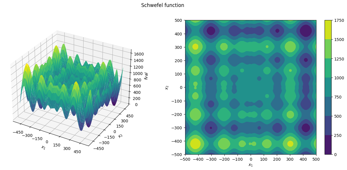
To run any optimization, we first need to specify the optimization problem. PyScat currently heavily relies on the pyPESTO framework and requires a pypesto.Problem. For this demo, we use the Schwefel function which is one of the examples included in PyScat:

from pyscat.examples import plot_problem, problem_info, xyz

cur_problem_info = problem_info["Schwefel"]

problem = cur_problem_info["problem"]

plot_problem(problem, title="Schwefel function")

# generate data for plotting
X, Y, Z = xyz(problem)


# plotting function for our objective landscape
def plot_f(ax=None):
    """contour plot"""
    if ax is None:
        ax = plt.gca()

    c = ax.contourf(X, Y, Z, cmap="viridis")
    plt.colorbar(c, ax=ax, label="fval")
    ax.set_xlabel("$x_1$")
    ax.set_ylabel("$x_2$")

Enhanced Scatter Search (eSS) — ESSOptimizer

The idea of ESS is to maintain some reference set (RefSet) comprising a constant number of points (dim_refset) that (a) explores the parameter space and (b) approaches minima.

The basic steps of ESS are:

• Initialization: Generate a diverse set of points in the parameter space.

• Recombination: Generate new points by recombining the RefSet.

• Improvement: Improve the RefSet by replacing points with better ones.

The steps are repeated until a stopping criterion is met.

ESS itself is gradient-free, but if gradient information is available, a gradient-based local optimizer can be used during the Improvement step (see below).

Initialize ESS

Create the initial RefSet:

• Sample n_diverse points

• Fill half of the RefSet with the best points

• Fill the other half with random points

# number of points in the RefSet
# (chosen for visualization, not a general recommendation)
REFSET_SIZE = 8
N_DIVERSE = 2 * REFSET_SIZE

# just some object that will evaluate
# the objective function and help us sample random points
evaluator = FunctionEvaluator(problem)
# create initial population
x, fx = evaluator.multiple_random(N_DIVERSE)
order = np.argsort(fx)
# the first half of the refset is the best points
# the second half is randomly selected
order[int(REFSET_SIZE / 2) :] = np.random.permutation(
    order[int(REFSET_SIZE / 2) :]
)
x = x[order]
fx = fx[order]

# initialize RefSet
refset = RefSet(
    x=x[:REFSET_SIZE, :],
    fx=fx[:REFSET_SIZE],
    evaluator=evaluator,
)
refset

RefSet(dim=8, fx=[296.07146848407615 ... 1171.5265299782527])

# visualize initialization
fig, axs = plt.subplots(1, 2, sharex=True, sharey=True, figsize=(16, 6))

ax = axs[0]
plot_f(ax=ax)
ax.scatter(
    x[:REFSET_SIZE, 0],
    x[:REFSET_SIZE, 1],
    c="yellow",
    marker="*",
    label="Initial RefSet",
)
ax.scatter(
    x[REFSET_SIZE:, 0],
    x[REFSET_SIZE:, 1],
    c="red",
    marker=".",
    label="Dismissed",
)
ax.legend(loc="center left", bbox_to_anchor=(1.2, 1.1))
ax.set_title("Initialization – n_diverse")

ax = axs[1]
plot_f(ax=ax)
ax.scatter(
    x[:REFSET_SIZE, 0],
    x[:REFSET_SIZE, 1],
    c="yellow",
    marker="*",
    label="refset",
)
ax.set_title("Initialization – RefSet")

plt.show()

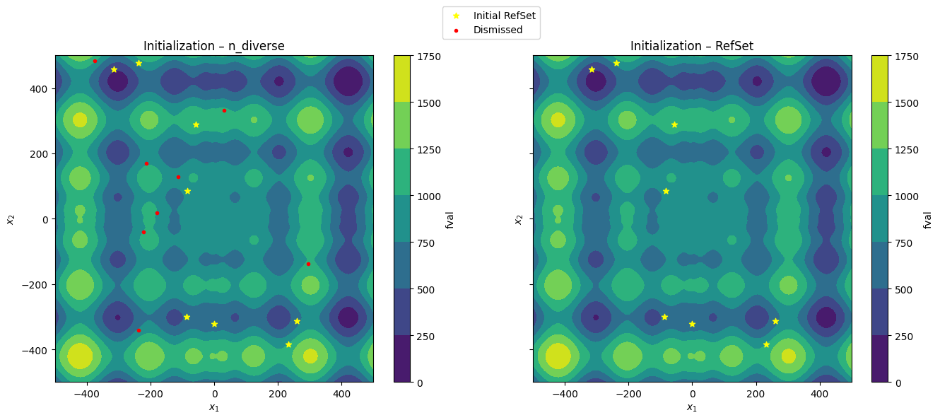
Hyperparameter controlling initialization:

• dim_refset: number of points in the RefSet

• n_diverse: number of initial random points to generate (default: 10 * dim_refset)

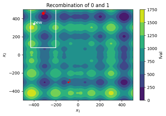
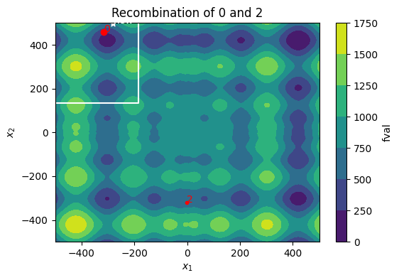
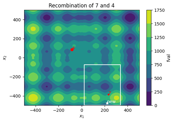
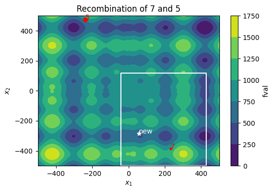
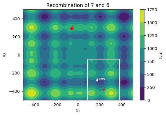
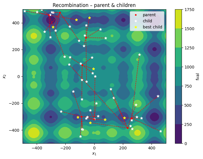
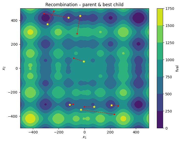
Recombination — generate new points based on the current RefSet

Every iteration generates \(dim\_refset^2 - dim\_refset\) new points from pairwise recombination of the RefSet members. Only the best offspring from each RefSet member will be retained. A new point can only replace its parent, but not any other RefSet member. This ensures that the RefSet remains diverse.

Currently, there are no hyperparameters to control recombination.

print(
    f"RefSet size if {refset.dim}. "
    f"Thus, recombination will generate {refset.dim**2 - refset.dim} "
    f"new points in each iteration."
)

RefSet size if 8. Thus, recombination will generate 56 new points in each iteration.

# Recombination scheme
from pyscat.ess import DefaultRecombination

recombinator = DefaultRecombination()
# for i, j in [(0, 8), (8, 0)]:
all_pairs = list(product(range(refset.dim), range(refset.dim)))
for i, j in all_pairs[:3] + all_pairs[-4:-1]:
    if i == j:
        continue
    c1, c2 = recombinator.get_hyper_rect(refset, evaluator, i, j)
    new_x = np.random.uniform(low=c1, high=c2, size=problem.dim)

    marker_i, marker_j = ("o", ".") if i < j else (".", "o")

    fig, ax = plt.subplots(figsize=(6, 4))
    plot_f(ax=ax)
    ax.scatter(x[i, 0], x[i, 1], c="red", marker=marker_i, label="refset")
    ax.text(x[i, 0], x[i, 1], str(i), color="red")
    ax.scatter(x[j, 0], x[j, 1], c="red", marker=marker_j, label="refset")
    ax.text(x[j, 0], x[j, 1], str(j), color="red")
    # draw the rectangle
    ax.plot(
        [c1[0], c2[0], c2[0], c1[0], c1[0]],
        [c1[1], c1[1], c2[1], c2[1], c1[1]],
        c="white",
    )
    # draw the new point
    ax.scatter(new_x[0], new_x[1], c="white", marker="*", label="new")
    # label the new point
    ax.text(new_x[0], new_x[1], "new", color="white")
    ax.title.set_text(f"Recombination of {i} and {j}")
    plt.show()
    print(f"#{i}: {problem.objective(x[i])}")
    print(f"#{j}: {problem.objective(x[j])}")

#0: 296.07146848407615
#1: 546.8969553152938

#0: 296.07146848407615
#2: 582.2267759729195

#7: 1003.1633178876884
#4: 839.4804068710703

#7: 1003.1633178876884
#5: 822.1189081863863

#7: 1003.1633178876884
#6: 1171.5265299782527

fig, ax = plt.subplots(figsize=(8, 6))
plot_f(ax=ax)

all_children = []
x_best_children = []
for i in range(refset.dim):
    children_i: list[np.ndarray] = []
    for j in range(refset.dim):
        if i == j:
            continue
        c1, c2 = recombinator.get_hyper_rect(refset, evaluator, i, j)
        new_x = np.random.uniform(low=c1, high=c2, size=problem.dim)
        children_i.append(new_x)
        # plot children with markers and plot line from parent to child
        ax.plot(
            [refset.x[i, 0], new_x[0]],
            [refset.x[i, 1], new_x[1]],
            c="red",
            linestyle="--",
            linewidth=1,
            zorder=1,
        )
        ax.scatter(new_x[0], new_x[1], c="white", marker="*", label="new")

    best_child_idx = np.array(
        [problem.objective(x) for x in children_i]
    ).argmin()
    ax.scatter(
        children_i[best_child_idx][0],
        children_i[best_child_idx][1],
        c="yellow",
        marker="*",
        label="new_best",
        zorder=10,
    )
    all_children.append(children_i)
    x_best_children.append(children_i[best_child_idx])

    ax.scatter(
        refset.x[i, 0],
        refset.x[i, 1],
        c="red",
        marker=".",
        label="refset",
        zorder=5,
    )

plt.legend(
    [
        plt.Line2D([0], [0], marker=".", c="red", linestyle="None"),
        plt.Line2D([0], [0], marker="*", c="white", linestyle="None"),
        plt.Line2D([0], [0], marker="*", c="yellow", linestyle="None"),
    ],
    ["parent", "child", "best child"],
)
plt.title("Recombination – parent & children")


# new plot with parents and best children connected by lines
fig, ax = plt.subplots(figsize=(8, 6))
plot_f(ax=ax)
for i in range(refset.dim):
    ax.plot(
        [refset.x[i, 0], x_best_children[i][0]],
        [refset.x[i, 1], x_best_children[i][1]],
        c="red",
        linestyle="--",
        linewidth=1,
        zorder=1,
    )
    ax.scatter(
        x_best_children[i][0],
        x_best_children[i][1],
        c="yellow",
        marker="*",
        label="new_best",
        zorder=10,
    )
    ax.scatter(
        refset.x[i, 0],
        refset.x[i, 1],
        c="red",
        marker=".",
        label="refset",
        zorder=5,
    )
plt.title("Recombination – parent & best child")

x_best_children = np.array(x_best_children)
fx_best_children = np.array([problem.objective(x) for x in x_best_children])

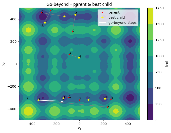
Go-beyond

The go-beyond strategy aims at improving the best children from recombination. If the offspring is better than the parent, the offspring will be used as the new parent for the next iteration. The offspring will be generated by sampling from a hyper-rectangle around the parent. The size of the hyper-rectangle is determined by the relative improvement of the offspring over the parent. The process is repeated until no further improvement is possible.

# Re-implementation of the go-beyond strategy
# because we need some internal state
def go_beyond(
    x_best_children: np.ndarray,
    fx_best_children: np.ndarray,
    refset: RefSet,
    evaluator: FunctionEvaluator,
) -> tuple[list[np.ndarray], list[np.ndarray], list[list[tuple[np.ndarray]]]]:
    trials_x = []
    trials_fx = []
    rects = []
    for i in range(refset.dim):
        cur_trials_x = [x_best_children[i][np.newaxis, :]]
        cur_trials_fx = [fx_best_children[i]]
        cur_rects = []

        if fx_best_children[i] >= refset.fx[i]:
            # include child before go-beyond,
            # since x_best_children will be updated here
            trials_x.append(cur_trials_x)
            trials_fx.append(cur_trials_fx)
            continue

        # offspring is better than parent
        x_parent = refset.x[[i]].copy()
        fx_parent = refset.fx[i]
        x_child = x_best_children[[i]].copy()
        fx_child = fx_best_children[i]
        improvement = 1
        # Multiplier used in determining the hyper-rectangle from which to
        # sample children. Will be increased in case of 2 consecutive
        # improvements.
        # (corresponds to 1/\Lambda in [Egea2009]_ algorithm 1)
        go_beyond_factor = 1
        while fx_child < fx_parent:
            # update best child
            x_best_children[i] = x_child
            fx_best_children[i] = fx_child

            # create new solution, child becomes parent
            # hyper-rectangle for sampling child
            box_lb = x_child - (x_parent - x_child) * go_beyond_factor  # if
            box_ub = x_child
            # clip to bounds
            ub, lb = evaluator.problem.ub, evaluator.problem.lb
            box_lb = np.fmax(np.fmin(box_lb, ub), lb)
            box_ub = np.fmax(np.fmin(box_ub, ub), lb)
            # sample parameters
            x_new = np.random.uniform(low=box_lb, high=box_ub)
            cur_rects.append(
                (box_lb, box_ub),
            )
            x_parent = x_child
            fx_parent = fx_child
            x_child = x_new
            fx_child = evaluator.single(x_child)
            cur_trials_x.append(x_child)
            cur_trials_fx.append(fx_child)
            improvement += 1
            if improvement == 2:
                go_beyond_factor *= 2
                improvement = 0
        trials_x.append(cur_trials_x)
        trials_fx.append(cur_trials_fx)
        rects.append(cur_rects)
    trials_x = list(map(np.vstack, trials_x))
    trials_fx = list(map(np.array, trials_fx))
    return trials_x, trials_fx, rects


trials_x, trials_fx, go_beyond_rects = go_beyond(
    x_best_children, fx_best_children, refset, evaluator
)
assert len(trials_x) == len(trials_fx) == refset.dim

# new plot with parents and best children connected by lines
fig, ax = plt.subplots(figsize=(8, 6))
plot_f(ax=ax)
for i in range(refset.dim):
    # line from old refset member to the best child from recombination
    ax.plot(
        [refset.x[i, 0], trials_x[i][0][0]],
        [refset.x[i, 1], trials_x[i][0][1]],
        c="grey",
        linestyle="-",
        linewidth=1,
        zorder=1,
    )

    # final points after go-beyond
    ax.scatter(
        x_best_children[i][0],
        x_best_children[i][1],
        c="yellow",
        marker="*",
        label="new_best",
        zorder=10,
    )

    # before go-beyond
    ax.scatter(
        refset.x[i, 0],
        refset.x[i, 1],
        c="red",
        marker=".",
        label="refset",
        zorder=5,
    )
    ax.text(refset.x[i, 0], refset.x[i, 1], str(i))

    # the go-beyond line
    ax.plot(
        trials_x[i][:-1, 0],
        trials_x[i][:-1, 1],
        linestyle="-",
        c="white",
        marker=".",
        zorder=1,
        linewidth=1,
    )
    for x, y in trials_x[i]:
        if problem.objective([x, y]) < refset.fx[i]:
            # ax.scatter(x, y)
            ax.text(x, y, str(i))

plt.title("Go-beyond – parent & best child")
plt.legend(
    [
        plt.Line2D([0], [0], marker=".", c="red", linestyle="None"),
        plt.Line2D([0], [0], marker="*", c="yellow", linestyle="None"),
        plt.Line2D([0], [0], marker=".", c="white", linestyle="-"),
    ],
    ["parent", "best child", "go-beyond steps"],
)
plt.show()

Local search (optional)

If a local optimizer is provided (local_optmizer), one of the current solutions may be improved further during each eSS iteration. This is heavily controlled by hyperparameters:

• whether a local search will take place at all:

  • local_n1: The number of eSS iterations after which the first local search will take place

  • local_n2: The number of eSS iterations that have to pass after the previous local optimization

• which solution will be optimized:

  • balance \(\in [0, 1]\): A priority score will be calculated for each RefSet member based on 1) its function value rank 2) its rank-based distance to previous local optimization results. balance determines the relative weight of (1) and (2) — a lower value favors quality, a higher value favors diversity.

Replacement of stuck RefSet members

If there was no improvement of a specific RefSet member during recombination, go-beyond, or local optimization over n_change (default: 20) iterations, the respective RefSet member will be replaced by a random point.

Full example

Run a ESSOptimizer optimization and show the results:

# Initialize and run the optimizer
ess = ESSOptimizer(max_eval=5000, dim_refset=10)
result = ess.minimize(problem)
result

<pypesto.result.result.Result at 0x7f3c0576fcb0>

# Show the optimization result
display_markdown(result.summary().replace("#", "##"), raw=True)

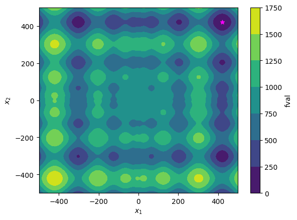
# Visualize the optimum
plot_f()
plt.scatter(
    result.optimize_result.x[0][0],
    result.optimize_result.x[0][1],
    c="magenta",
    marker="*",
    label="Reported optimum",
)
plt.show()

Optimization Result

• number of starts: 1

• best value: 5.7918300967685354e-05, id=0

• worst value: 5.7918300967685354e-05, id=0

• number of non-finite values: 0

• execution time summary:

  • Mean execution time: 0.263s

  • Maximum execution time: 0.263s, id=0

  • Minimum execution time: 0.263s, id=0

• summary of optimizer messages:

  Count	Message
  1	Global best

• best value found (approximately) 1 time(s)

• number of plateaus found: 0

A summary of the best run:

Optimizer Result

• optimizer used: <pyscat.ess.ESSOptimizer object at 0x7f3c0576fe00>

• message: Global best

• number of evaluations: 5005

• time taken to optimize: 0.263s

• startpoint: None

• endpoint: [420.95716836 420.97984678]

• final objective value: 5.7918300967685354e-05

assert (
    abs(cur_problem_info["global_best"] - result.optimize_result.fval[0])
    < 1e-3
)

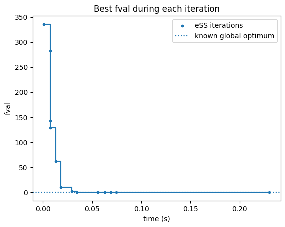
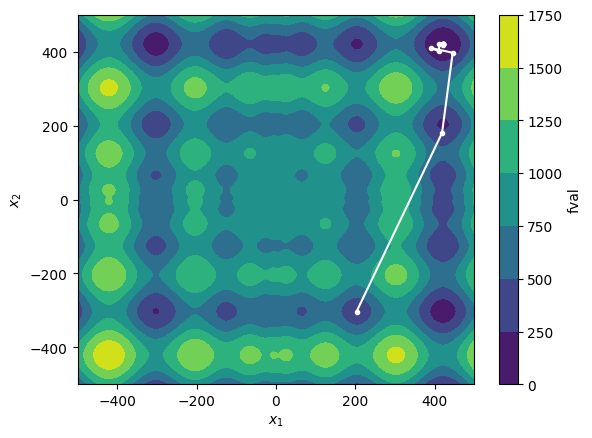
Visualize optimizer trajectory across iterations:

from pyscat.plot import plot_ess_history

plot_ess_history(ess.history)
plt.axhline(
    cur_problem_info["global_best"],
    linestyle="dotted",
    label="known global optimum",
)
plt.legend()
plt.show()

plot_f()
h = np.vstack(ess.history.get_x_trace())
plt.plot(h[:, 0], h[:, 1], marker=".", c="white")
plt.show()

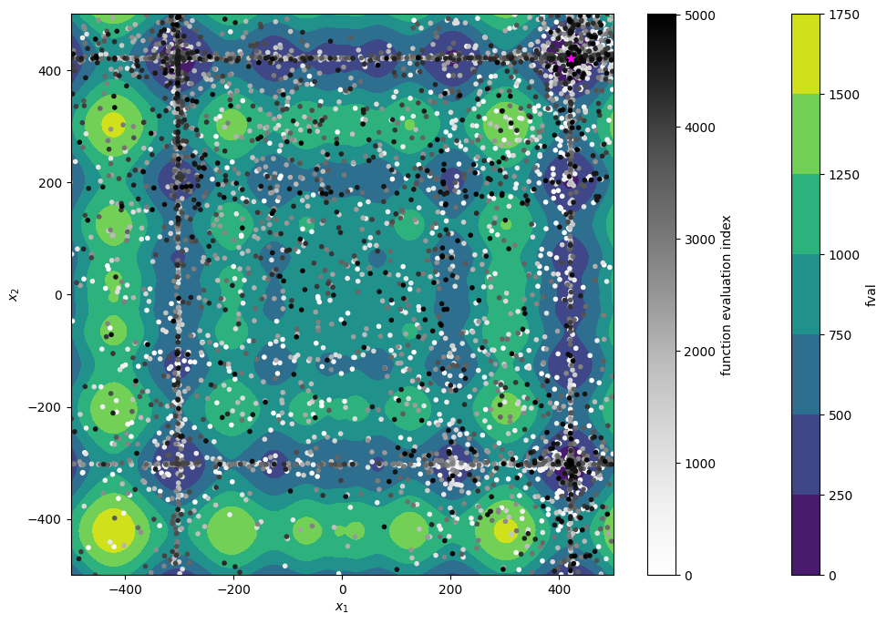
Let’s look at the exploration of the parameter space:

# show exploration of the parameter space
problem.objective.history = MemoryHistory()
ess = ESSOptimizer(max_eval=5000, dim_refset=10)
result = ess.minimize(problem)
x_trace = np.vstack(problem.objective.history.get_x_trace())
fval_trace = np.vstack(problem.objective.history.get_fval_trace())
problem.objective.history = NoHistory()

plot_f()
plt.scatter(
    x_trace[:, 0],
    x_trace[:, 1],
    c=np.arange(len(x_trace)),
    cmap="Greys",
    marker=".",
    label="function evaluation",
    alpha=1,
)
plt.scatter(
    result.optimize_result.x[0][0],
    result.optimize_result.x[0][1],
    c="magenta",
    marker="*",
    label="Reported optimum",
)
plt.gcf().set_size_inches(12, 8)

# add color bar for function evaluations, normalize to length
cbar = plt.colorbar(
    plt.cm.ScalarMappable(
        cmap="Greys", norm=plt.Normalize(vmin=0, vmax=len(x_trace))
    ),
    ax=plt.gca(),
)
cbar.set_label("function evaluation index")
plt.show()

General hyperparameters for ESSOptimizer

• parallelization of objective evaluation (mutually exclusive):

  • n_procs: Number of processes for multiprocessing-based parallelization

  • n_threads: Number of threads for threading-based parallelization

• exit criteria:

  • max_eval: Maximum number of objective evaluations

  • max_walltime_s: Maximum walltime (seconds)