Getting started with SacessOptimizer

A short introduction to using the self-adaptive cooperative enhanced scatter search (saCeSS) implementation from pyscat for global optimization.

Setting up the optimization problem

pyscat builds on top of pypesto and thus requires a pypesto.Problem instance to define the optimization problem. Here, we create a simple test problem using the Rosenbrock function.

import logging

import numpy as np
from pypesto import Problem
from pypesto.objective import Objective
from scipy.optimize import rosen, rosen_der

# Create an objective function based on the Rosenbrock function
objective = Objective(fun=rosen, grad=rosen_der)

# Define the optimization problem with bounds
problem = Problem(
    objective=objective,
    # SacessOptimizer requires finite bounds on all estimated parameters
    lb=0 * np.ones((1, 2)),
    ub=1 * np.ones((1, 2)),
)

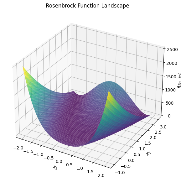
Let’s visualize the Rosenbrock function to get an idea of the optimization landscape:

import matplotlib.pyplot as plt


def plot_rosenbrock():
    x = np.linspace(-2, 2, 400)
    y = np.linspace(-1, 3, 400)
    X, Y = np.meshgrid(x, y)
    Z = rosen(np.array([X, Y]))
    fig = plt.figure(figsize=(10, 7))
    ax = fig.add_subplot(111, projection="3d")
    ax.plot_surface(X, Y, Z, cmap="viridis", alpha=0.8)
    ax.set_xlabel("$x_1$")
    ax.set_ylabel("$x_2$")
    ax.set_zlabel("$f(x_1, x_2)$")
    ax.set_title("Rosenbrock Function Landscape")
    plt.show()


plot_rosenbrock()

Running the optimization

We can now set up and run the SacessOptimizer. saCeSS has a variety of hyperparameters that can be tuned to improve optimization performance. Here, we will use the default settings for simplicity.

Two settings are mandatory for SacessOptimizer: the number of workers, i.e., parallel processes, and the walltime for the optimization.

from pyscat import SacessOptimizer

# Initialize the SacessOptimizer
optimizer = SacessOptimizer(
    problem=problem,
    # The minimum number of workers is 2, but using more is recommended
    num_workers=8,
    # For this simple example, a couple of seconds is sufficient
    max_walltime_s=1,
    # Disable verbose output for cleaner output
    sacess_loglevel=logging.WARNING,
)

# Run the optimization
res = optimizer.minimize()

The optimization result is stored in a pypesto.Result object. We can inspect the best found parameter values and the corresponding objective function value:

best_x = res.optimize_result[0].x
best_fval = res.optimize_result[0].fval
print(f"Best parameters found: {best_x}")
print(f"Objective function value at best parameters: {best_fval}")

Best parameters found: [1. 1.]
Objective function value at best parameters: 0.0

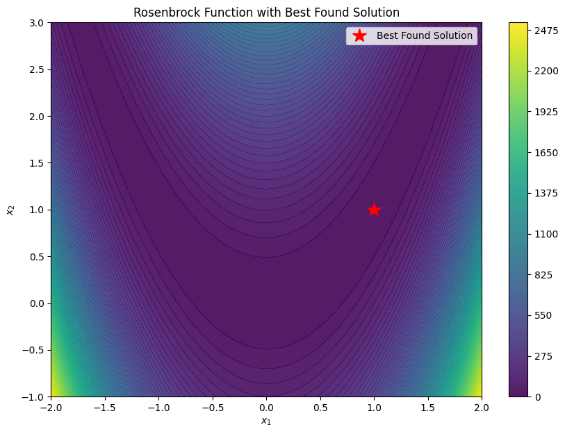
We can graphically confirm that the optimizer found a good solution by plotting the Rosenbrock function and marking the best found parameters:

# Visualize the optimization result
x = np.linspace(-2, 2, 400)
y = np.linspace(-1, 3, 400)
X, Y = np.meshgrid(x, y)
Z = rosen(np.array([X, Y]))
fig, ax = plt.subplots(figsize=(10, 7))
contour = ax.contourf(X, Y, Z, levels=100, cmap="viridis", alpha=0.9)
plt.colorbar(contour)
ax.plot(best_x[0], best_x[1], "r*", markersize=15, label="Best Found Solution")
ax.set_xlabel("$x_1$")
ax.set_ylabel("$x_2$")
ax.set_title("Rosenbrock Function with Best Found Solution")
ax.legend()
plt.show()

This concludes our brief introduction to using the SacessOptimizer from pyscat for global optimization tasks. For more advanced usage and hyperparameter tuning, please refer to the pyscat documentation. For more information on pypesto, such as problem definition and storage of results, please refer to the pyPESTO documentation.